Count-Min Sketching, Configuration & Point-Queries

A probablistic counting algorithm, implementation, configuration, and application notes.

DRAFT

Introduction

Sketching algorithms like this one are the heart of many stream processing applications for good reason. Sketches can produce estimates of configurable quality, require requires sub-linear space and often do not need to store identifiers. This makes them an attractive option for counting a large number of distinct items with relatively little space.

The Count-Min Sketch is a probablistic sketching algorithm that is simple to implement and can be used to estimate occurrences of distinct items. This article will give you a hands-on walk through of how this works in a live demo, and explaination of how to configure your own sketch.

Sketches

A sketch of a matrix A is another matrix B which is signiﬁcantly smaller than A, but still approximates it well.

Theory

This section outlines brief summary of the important properties of this sketch. I'll try to provide an explaination of what these properties mean without getting bogged down in mathematical proofs so that you'll be able to reason about sketch behavior and configuration.

The theory behind this particular stream summary was first described by Graham Cormode in "Count-Min Sketch".

Model

A few simple equations are used to model this sketch:

U: a (possibly large) universe of possibilities
x: x ∈ U, set x selected from universe of U
δ: error probability (delta)
ε: error factor (epsilon)
f_(x): true number of occurrences of x

The sketch can be defined as:

f '_(x): estimated number of occurrences of x

Guarantee

Cormode proved the sketch provides the guarantee that with probability 1 - δ:

f_(x) <= f '_(x)
truth <= estimate

This means that the sketch never under-estimates the true value, though it may over-estimate.

Cormode also proved the sketch provides the guarantee that with probability 1 - δ:

∥f∥ = Σ_{x ∈ U} f_(x)
f '_(x) <= f_(x) + ε∥f∥
estimate <= truth + error

This means that amount of error in the estimate is proportional to the total aggregate number of occurences seen, and to the epsilon. This also means significantly larger truth values can dwarf smaller the error term producing more accurate estimates for items with the largest counts.

Finally, the theory provides a few formulas for determining the dimensions of the array used to store estimates.

width: ⌈e / ε⌉
depth: ⌈ln 1 / δ⌉

Implementation

This section provides a short description of the algorithm and illustrations of operations on the underlying data structures. Given a configuration:

δ: error probability (delta)
ε: error factor (epsilon)

Setup

This requires O((1 / ε) * ln(1 / δ)) space.

Create an array with the width and depth, given above, initialize to zero.
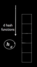
Create a set of size depth universal hash functions, { h₁ ... h_d ... h_depth }.

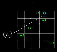
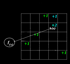
Increment

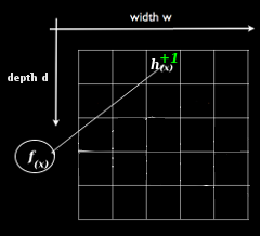
This requires O(ln(1 / δ)) time. For each level of depth, d in [0, depth):

Apply the hash h_d to the value of x, modding it with the width to generate a column number. col = h_d(x) % width
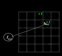
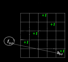
Increment the count, storage[d, col]++

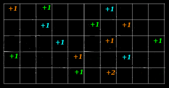
Below is an illustration of the hash functions on the leftmost diagram, and on the rest, sketch increments at increasing levels of depth (from left to right):

. . .

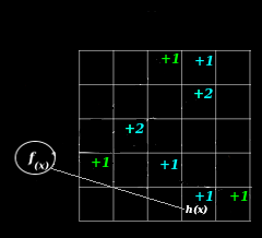
Collisions And Epsilon

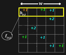
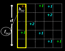
Collisions are one source of error in the estimates a sketch can produce. Below is an illustration, a hash function is selected on the left and a collision occurs during an update on the right. The net result is that the estimate contains counts that are higher than the true value.

. . .

Modeling Error Impact

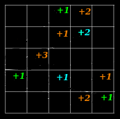
Intuitively, it's easy to understand how collisions result in a value higher than the actual value. You can see this in the illustration above in cells containing a +2. The notion of over-counting is also reflected in the model:

f_(x) <= f '_(x)

Intuitively, it's easy to imagine how counting one more item to the example could result in more collisions, creating more overcounting, creating more +2s, and even some +3s, when no item ever appeared more than once. The notion that adding things to the sketch can increase the amount of error in any single estimate can be seen in the model, too:

f '_(x) <= f_(x) + ε∥f∥

The value of ∥f∥ is calculated by summing all of the counts together, adding more data naturally makes ∥f∥ bigger, increasing the error term, ε∥f∥.

More Collisions

Wider Sketch - Fewer Collisions

Configuring Epsilon

One strategy for reducing the amount of over-estimation is to hash into more buckets. The theory gives us a formula to describe the number of buckets used:

width: ⌈e / ε⌉

The value of ε is inversely proportional to the width of the sketch, so choosing a smaller ε would result in a wider sketch.

f '_(x) <= f_(x) + ε∥f∥

The error term for the estimate depends on ε, and is directly proportional to the amount of error in the estimate. Choosing a smaller ε would help reduce the over all error term, ε∥f∥.

The fact that more buckets requires more space is reflected in the O((1 / ε) factor of the space requirements.

Probability And Delta

Modeling Error Rate

At a high level this algorithm involves fitting n items into m buckets. The expected probablity of error would be number of items (n) / number of buckets (m):

Pr(collision) = n / m (simple hashing)

Pr(collision) <= 1 / n (pairwise independent hashing)

With a single hashing function, Pr(collision) can rise dramatically with large values of n. Universal hashing is a technique for maintaining lower Pr(collision) by randomly selecting a set of hash functions:

Pr(collision) <= 1 / m (universal hashing)

width = single trial

depth = # of indepedent trials

Configuring Delta

Choosing a value of δ allows you to select a desired probability of error, Pr(desired). Pr(collision) is a function of the width of each row in the array, and may be a different and smaller than your Pr(desired) since width is chosen with different considerations.

δ = Pr(desired)
δ = Pr(desired) >= Pr(collision)

The familiy of universal hashes is also a familiy of independent hashes. This means that we can combine results from different independent trials. Each independent trial becomes a level of depth in the array.

δ = Pr(desired) <= depth * Pr(collision)

Trials are repeated until enough are completed to achieve the Pr(desired), this is why the main loop in the algorithm is revolves around the depth of this array.

Querying

Point-Query

Looking up the value of a counter in the sketch is the simplest type of query called a point-query. This proceedure is very similar to the increment proceedure and also requires O(ln(1 / δ)) time.

Set your initial result to ∞, then for each level of depth, d in [0, depth):

Apply the hash h_d to the value of x, modding it with the width to generate a column number. col = h_d(x) % width.
Keep the minimum, result = min(result, storage[d][col]).

Complexity

Space

The width and depth of the array used to store the occurence estimates is given by:

Space Used = O((1 / ε) * ln(1 / δ))

Generally speaking, arrays will be wider than they are deep in most practical configurations (e.g. epsilon = 0.0001, delta = 0.95 :: width = 27183, depth = 3).

Time

During reads and writes, the depth of the array dictates the number of hashes that are ultimately performed.

Time Needed = O(ln(1 / δ))

Configuration

When choosing a configuration, you are often trying to minimize the error term, ε∥f∥, of the estimate:

Epsilon: Acceptable errors in estimation fall within a range which is a factor of ε. Smaller values of ε should produce sketch configurations that provide estimates closer to the true values. However, this will increase the space required by the sketch.
Volume: Error in estimation is also proportional to the total number of distinct items counted. A factor in the error term, ∥f∥, is a summation of total number of occurences of each distinct item. Another way to reduce the error term is to reduce ∥f∥ by counting fewer things.

Alternatively, you can try to reduce the frequency error and increase the chance of success, (1.0 - δ). You may trade some level of error rate in the estimate for a savings in space:

Delta: The theory states that errors in estimation occur with probability of delta (δ). This makes the probability of success (1.0 - δ). Increasing this number can produce sketch configurations with reduced error rates, but that will require more memory.

Universal hashes?

Seed: The seed parameter controls the distribution of universal hash functions that are used by the sketch.

A good rule of thumb for finding a starting configuration is to try an epsilon with as many significant digits as you have digits in your expected volume (e.g. given an expected volume of 5000 a good starting point for epsilon might be .0001).

Calculator

The following calculator allows you to visualize how the estimated and true values produced by these functions relate to one another for various configurations. In this scenario, a set of random counts are generated and assigned to each key in a set of keys. Points are colored red to show when they are outside a factor of epsilon of the true value. For reference, a perfect estimate would look like a diagonal line, from the bottom left to the top right and would contain no red.

Truth (x-axis) vs. Estimate (y-axis)

Source Code: cmsketch.js

Saturation

A sketch is said to be saturated when it's filled with data, and adding additional data to the sketch at this point has a high likihood introducing error. Recall the error model for the sketch, it's proportional to the volume and cardinality of the data added to the sketch, ∥f∥ in the expression below.

f '_(x) <= f_(x) + ε∥f∥

Keeping track of the count of the number of items added to a sketch is allows you to track volume, and assuming the cardinality of the items your sketch sees stays within your estimated limit, this gives you one way to estimate how saturated a sketch is. Once you know your sketch is saturated you should stop adding data to it, and start using a new sketch. Alternatively, you might accept the error and log an error or emit some metric.

For more on embracing probability and error, see Count-Min Sketching, Saturation & Heavy-Hitters

Author

Eric Crahen